He meant it as a fun idle topic of conversation, but somehow I couldn’t get this idea out of my head, and ended up running with it…and running…and running…and now I’ve built Nodariety.jl. It contains a ton of data I curated detailing a huge list of hyphenated theories (or theorems, or experiments, etc. etc.) and structuring this data into a directed graph.

In this post, I’ll give some details on what the package does, some results of my own playing around with this really fun hobby project, and also ways you can contribute if you’re so inclined! And for the answer to the original question of what the longest path was, read on… 😉

What do you get?

The package does a few things:

1. Defines a HyphenGraph type, which is <:LightGraphs.AbstractGraph, stores the graph itself as a MetaGraphs.MetaDiGraph object, as well as the node and edge data as DataFrames.
2. Defines a default instance of this type, exported as the variable hg, which as of this writing, includes 446 nodes and 383 edges.
3. Exports a function for visualizing the graph with nodes and edges colored and labeled according to various pieces of data (see some examples of this below).
4. Exports some graph analysis and demographic plotting functions (again, examples below).

The package is registered in the Julia General registry, so you can install it easily via ] add Nodariety and have all of these things in your own REPL to play around with! 😀

Playing around!

Here’s a first visualization of the graph, resulting from the command plot_graph(node_color_prop="birth_year", edge_color_prop = "year"). It uses one unified color scheme, ranging from red to green, to indicate the birth years of people at the nodes, and the year of reference for the theories on the edges:

There are a lot of isolated clusters here, which make things hard to reason about. Let’s get just the largest connected cluster…

julia> cs = get_clusters() # get all connected clusters
 [1, 4, 6, 12, 15, 18, 21, 26, 27, 28  …  419, 427, 428, 430, 435, 437, 441, 443, 444, 446]
 [13, 57, 80, 106, 113, 121, 124, 165, 200, 239  …  298, 314, 315, 325, 333, 340, 350, 359, 381, 403]
 [2, 19, 55, 101, 125, 140, 146, 190, 201, 203, 205, 218, 276, 305, 351, 358, 374, 423]
 [8, 9, 16, 88, 149, 170, 254, 287, 328, 352, 367, 383, 398, 399, 402]
 [32, 51, 151, 171, 187, 221, 230, 275, 310, 311, 343, 408, 413]
 [63, 112, 152, 216, 225, 229, 265, 332, 382, 396, 442, 445]
 [5, 127, 175, 179, 181, 346, 363, 373]
 [10, 47, 83, 184, 263, 300, 324, 356]
 [195, 227, 271, 274, 301, 318, 376, 406]
 ⋮
 [294, 429]
 [307, 432]
 [308, 394]
 [322, 345]
 [327, 371]
 [349, 405]
 [375, 440]
 [393, 438]
 [395, 424]

julia> sg = hg[cs[1]] # could also do trim_graph(threshold=100)
HyphenGraph with 248 people, 251 hyphens

julia> julia> plot_graph(sg, node_color_prop="birth_year", edge_color_prop="year")

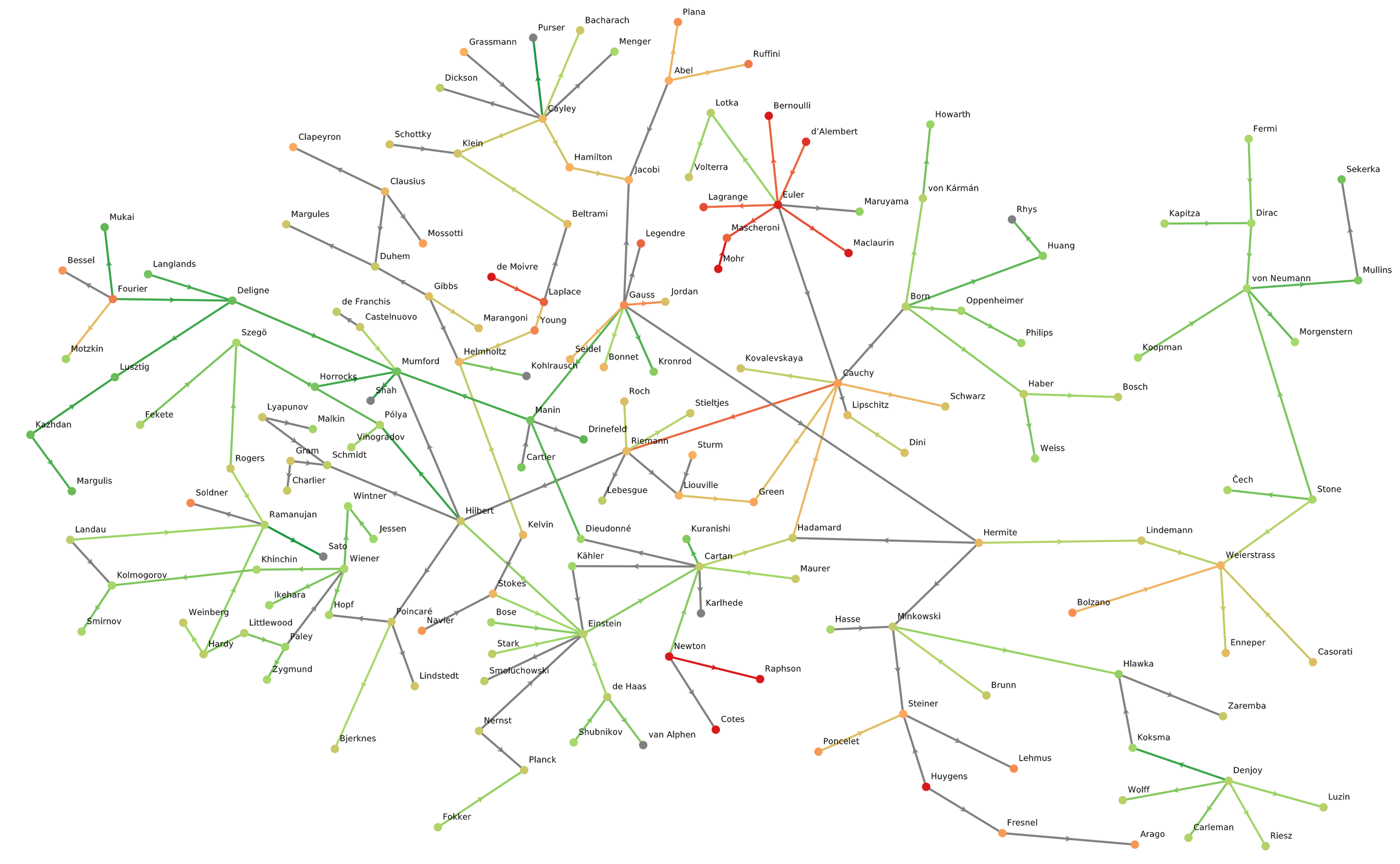
The GLMakie visualization is interactive, so I did some manual rearranging of the node positions to make this more visually parse-able…see “how you can help” below).

We could also color nodes by other properties such as various demographic properties, but some of those are a bit easier to parse if we just look at some histograms. For that, there’s a node_histogram function. For example, node_histogram(“gender”) yields:

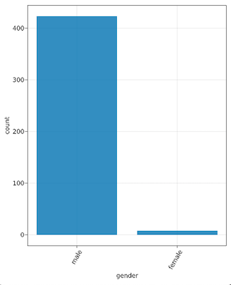
Pretty depressing. Even more so if you then try node_histogram(“given_name”), at which point you can find which three male names have more instances than the total number of women. Similar results from node_histogram("birth_continent")…

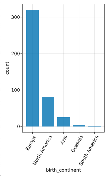
Obviously, a lot of this reflects historical norms and precedents, but it’s a pretty dramatic representation of how we can and need to do better going forward as a community. (It also, perhaps, suggests opportunities for targeted Wikipedia content-creation campaigns!)

But let’s try something else fun! Because HyphenGraph<:AbstractGraph, lots of LightGraphs functionality “just works” here (in fact we’ve already used it to find clusters above), so we can do neat stuff like probe centrality measures. I’ve included some functions for this:

julia> most_central(betweenness_centrality) # get details for one measure
Dict{Symbol, Any} with 9 entries:
  :birth_year      => 1879
  :given_name      => "Albert"
  :death_year      => 1955
  :birth_country   => "Germany"
  :race            => "white"
  :reference       => "https://en.wikipedia.org/wiki/Albert_Einstein"
  :birth_continent => "Europe"
  :family_name     => "Einstein"
  :gender          => "male"

julia> all_centrals() # or just do a bunch of them!
betweenness_centrality: Albert Einstein
closeness_centrality: Leonhard Euler
degree_centrality: Albert Einstein
eigenvector_centrality: Satyendra Bose
katz_centrality: David Mumford
pagerank: Albert Einstein
stress_centrality: Albert Einstein
radiality_centrality: Niels Abel

Or, we can answer the question that started it all…

julia> paths = longest_path() # get indices of paths
2-element Vector{Vector{Int64}}:
 [183, 391, 82, 40, 75, 248, 282, 368]
 [285, 391, 82, 40, 75, 248, 282, 368]

julia> hg[paths[1]].node_info.family_name
8-element Vector{String}:
 "Kelvin"
 "Stokes"
 "Einstein"
 "Cartan"
 "Dieudonné"
 "Manin"
 "Mumford"
 "Shah"

julia> hg[paths[2]].node_info.family_name
8-element Vector{String}:
 "Navier"
 "Stokes"
 "Einstein"
 "Cartan"
 "Dieudonné"
 "Manin"
 "Mumford"
 "Shah"

How can you help?

In plenty of ways! Some ideas to start with:

1. Add more data! The best way to do this is by GitHub pull request. While it’s not absolutely required, I would strongly request that if you do this, you follow these guidelines:
   1. Chase tails thoroughly. e.g. if you want to add the A-B theorem, but A is also part of the A-C conjecture, the D-A algorithm, etc., make sure to add those (and so on down the branches).
   2. Add as much data as you can find (leave minimal missing entries in the CSV files); try to at least exhaust Wikipedia’s resources.
   3. Please include open-access references in those fields.
2. Help with graph layout! You may notice that there are lots of edge crossings in the plots above. I’ve played around with a variety of layout algorithms from the NetworkLayout.jl package, but none of them are quite satisfactory. If you’re handy with that sort of thing, feel free to help!
3. Other visualization help! I have an alternative approach to graph visualization that you can see at Nodariety (GitHub repo here) that has some nice things about it; in particular the little popups with other information. Would be cool to figure out a non-laggy way to do that within GraphMakie…
4. Try out other fun ideas for graph analysis and make PR’s with those functions!

I very much hope people might find this as rewarding of a hobby pursuit as I’ve found it to be, and would very much welcome any and all contributions! Please check out the issues on the repository for some more specific suggestions, as well!

(One BBC article puts forward the arguably contrarian take that it could be a good thing because it stimulates creativity or something, but let’s set that aside as an outlier and roll with the assertion that most of the time, multitasking is bad.)

Here’s the thing. As plenty of these articles point out, everything being on Zoom makes it so. damn. tempting. Especially if everyone’s cameras are off anyway, or it’s a webinar. Especially if the discussion is not particularly interesting or engaging. Especially if the to-do list is intimidatingly long. It’s absolutely tantalizing to just cruise through some emails or other minor chores. And probably sometimes that’s fine. (We all have things that we feel some obligation to be “present” at, but don’t get much from.)

But lately, I’ve realized that it’s actually been a long time since I gave my full attention to the entire duration of a webinar, conference talk, or even just large meeting that I wasn’t actively leading or participating in, and that strikes me as a problem. After all, in an in-person department seminar, I’m very rarely if ever on my laptop or otherwise trying to do anything other than listen to the speaker. And sometimes, it could be a talk that I would’ve been really interested in, but because I let myself be distracted at the beginning, I lost the thread.

So in the name of personal accountability, but also because I suspect I’m not the only one experiencing this, I’m going to posit some relatively specific measures that might help start to address this, mainly by reducing the temptation to turn my attention to other things. Some of them I already do somewhat regularly. Some are things I’d like to start doing, or start doing more of. Anyway, here goes.

1. Do things in fullscreen mode when possible. I already do this as a matter of course for tasks on which I can’t make any progress without undivided attention (coding, debugging, writing, etc.). I’d like to start doing it more for things like Zoom meetings, and maybe even temporarily turn off extra monitors that are only serving as distractions during those times.

2. Mitigate others’ expectations. For example, set a Slack status as “away” during meetings/talks and maybe even mute notifications to reduce the temptation to respond to messages that come in.

3. Take actual breaks. This one I’m actually alright at. When I feel my focus waning, I step away from my desk and go for a walk, make some tea, do some yoga, work out, or otherwise disconnect briefly. I do often succumb to the temptation to continue answering Slack messages or emails that come in during breaks, so I could probably do to incorporate the wisdom of #2 above into my practice of this.

I genuinely believe that not only will these things make me a happier and healthier person, but through doing so, will increase me efficiency and productivity, because without the mental overhead of constantly switching my attention, I can put in more hours of quality work in any given day.

Maybe you want to join me?

(Full disclosure: This post was written while I was “at” a poster session for a conference. But nobody came to see the poster during that time…)

Since I moved to Pittsburgh and have been cycling on some of the abundant hills in this area (I actually had to get some easier gears on my bike for this purpose), it’s been interesting to track all this data as I (oh so very gradually) get better at climbing! On my ride yesterday, I started getting curious about some of the inherent differences between riders with different FTP riding on the same terrain, and also the nonlinearities between power and speed, on those gradients or on a flat road. So I decided to do some physics to it!

The model

NOTE: Thanks a million to Chris White from Ride Far for this PDF that informed my notation here, and more importantly, provided some characteristic values for several of the coefficients about which I had no idea.

All the calculations I allude to below have been done in Python and the code is available on GitHub here, but I’ll include some of it inline in this post too. To start…

from scipy.constants import g, R, atm
import numpy as np
from itertools import product
import pandas as pd
import seaborn as sns
from matplotlib import pyplot as plt

Okay, so let’s lay out these equations. The basic premise of all of this (thanks, Newton) is that if you’re going at a steady speed, the power you are exerting should be equal to the power being dissipated by all the various resistive forces:

So the crux of this is modeling either side of this. Let’s start with the more complicated one, the right side. For this, we need to enumerate every resistive force. First, air resistance:

where $C_dA$ is the product of the drag coefficient and the area (characteristic values for this are tabulated here), $v_a$ is the air speed, and $\rho$ is the air density, which we can model as:

where $p_0$ is a standard atmosphere (101,325 Pa), $R_s$ is the specific gas constant (287.058 J/[kg K]), $L$ is the approximate rate of decrease in temperature with elevation (0.0065 K/m), $h$ is the altitude in meters (about 500 for Pittsburgh), $M$ is the molar mass of dry air (0.02896 kg/mol), and $R_U$ is the universal gas constant (8.315 J/[mol K]).

Here’s the Python code for air resistance:

# air density in kg/m^3
def air_density(altitude=500, T=293):
    L = 0.0065
    T0 = 298
    M = 0.02896
    Rs = 287.058
    p_exp = M*g/(R*L)
    p = atm*(1-(L*altitude/T0))**p_exp
    return p/(Rs*T)

# resisting force from air
def F_air(mph, CdA, rho=air_density()):
    speed = mph/2.237
    return 0.5 * CdA * rho * speed**2

Next, rolling resistance! To compute the rolling friction, we need to know the force normal to the road, hence the triggy stuff.

def F_roll(grad, m, Crr):
    return Crr * np.cos(np.arctan(grad)) * m * g

Here, $C_{rr}$ is the coefficient of rolling resistance (which I could look up for my tires here, it’s 0.00483), and $G$ is the gradient of the road, that is, the tangent of its angle of inclination.

And finally, gravity, for which we need the component along the level of the road:

def F_grav(grad, m):
    return np.sin(np.arctan(grad)) * m * g

We can sum these up and multiply by the ground speed to get the total resistive power:

I’ll also assume for simplicity that $v_g=v_a\equiv v$, i.e. the ground speed is equivalent to the air speed (no wind). Then, the above equation becomes a cubic in the velocity:

We’re almost there! We just need the other side of that original equation, the $P_{wheel}$ part. Unfortunately, all the power I can drive from my legs into my pedal-based power meter does not get to the wheel to drive the bike forward, because drivetrains are not 100% efficient. So we need to account for drivetrain losses $L_{dt}$:

Thanks to Chris White, I now know that a characteristic value for $L_{dt}$ is 0.051, so that’s what I’ve used here.

The results

First, I made a plot of power needed to achieve a given speed on various gradients (for reference, 0.0 is a flat road, 0.06 is usually the highest allowed on US highways, and the steepest hill in Pittsburgh (also the steepest public road in the US) is Canton Avenue which purportedly reaches a grade of 0.37):

def P_needed(mph, grad, m, CdA, Crr, rho, L_dt=0.051):
    speed = mph/2.237 # convert to m/s
    F_resist = F_air(mph, CdA, rho) + F_roll(grad, m, Crr) + F_grav(grad, m)
    return F_resist * speed / (1.0-L_dt)

mph_vals = np.arange(4,12.1,0.1)
grad_vals = np.arange(0.0, 0.25, 0.03)
df = pd.DataFrame.from_records(data=[p for p in product(mph_vals, grad_vals)], columns=["speed", "gradient"])
# calculate for me and my bike
df['W/kg'] = [Wperkg(63.5, 8.0, a.speed, a.gradient) for a in df.itertuples()]
sns.lineplot(x='speed', y='W/kg', data=df, hue='gradient', palette=sns.cubehelix_palette(len(grad_vals), start=0, rot=.5))
# plus some plot formatting stuff

Note that the y-axis here is in watts per kilogram of body mass, so things will shift a bit if the ratio of body mass to bike (+gear) mass changes, for the calculations here it was about a factor of 9. I also put my FTP and my maximum 5-second power on as reference points. The choice of x-axis lower limit was also deliberate, as in my experience, 4 mph is about the slowest one can go uphill and remain upright.

So this plot certainly shows some of the things I’d been thinking about – for example, if we consider FTP to be some measure of “sustainable” power output, then we can get a sense of what grades folks with different FTP values can sustainbly chug their way up for quite awhile while staying above that 4mph threshold. For me at 2.24, it’s something like 9-10% or so. Whereas if you’re a much fitter person than I, you might be able to go up that 9% in excess of 10 mph at your FTP, or alternatively, at around the same pace on something like a 15% grade.

This is cool, but I realized I actually wanted a different chart, one where we could explicitly see the tradeoff between speed and gradient for a fixed power. To do that, we need to solve the cubic equation I outlined above. Fortunately, it always has exactly one real root, so that’s pretty easy, and we can make this plot (we’re essentially showing where different horizontal lines on the previous plot intersect with the curves for different gradients):

def calc_speed(watts_per_kg, grad, body_mass, bike_mass, CdA=0.45, Crr=0.00483, rho=air_density(), L_dt=0.051):
    total_mass = body_mass + bike_mass
    a3 = 0.5*CdA*rho
    a1 = F_roll(grad, total_mass, Crr) + F_grav(grad, total_mass)
    a0 = -1.0 * watts_per_kg*body_mass * (1.0-L_dt)
    rts = np.roots([a3, 0, a1, a0])
    # one should be real, return that one
    return [r.real*2.237 for r in rts if r.imag==0][0]

    P_vals = np.arange(1.0,22.1,3.0)
    grad_vals = np.arange(0.0,0.252,0.002)
    df = pd.DataFrame.from_records(data=[p for p in product(P_vals, grad_vals)], columns=["W/kg", "gradient"])
    df['mph'] = [calc_speed(a[1], a.gradient, 63.5, 8.0) for a in df.itertuples()]

sns.lineplot(x='gradient', y='mph', data=df, hue='W/kg', palette=sns.cubehelix_palette(len(P_vals), start=0.2, rot=1.0))
# plus some more beautification

(Sidenote: Cubehelix color palettes are so cool! As is Seaborn generally for dataviz.)

Here now I’ve overlaid my own FTP, maximum 1-minute, and maximum 5-second power values as additional iso-lines. Again, the minimum speed shown is 4mph. For some typical numbers for male and female cyclists of various calibers, check out the chart partway down this page.

In this plot, it’s even easier to read off the kind of things I was discussing above, and also to draw conclusions about what kind of gradients one could “power up” for really short periods of time. For example, if your absolute maximum power output were 4 W/kg, you’re not going to be able to get up anything steeper than around 19%, even instantaneously.

All this analysis is cool, and also serves as a good motivator to get out and improve my power numbers! Especially since the iso-power slopes at the bottom of this curve are such that a relatively small improvement in power capability leads to a comparatively large one in accessible gradients, and I’d love to take a shot at the Dirty Dozen someday!

Reminder that the code is all here so you should definitely go play and put in your own numbers to see how this turns out for you!

Caveats!

In any simple model like this, there are a lot of assumptions! Here is a not-necessarily-exhaustive list

• I ignored the effects of wind (as mentioned above, assumed ground speed equal to air speed)
• I assumed perfectly smooth power profiles, which really only happens if you have ideal pedaling technique – in reality, most of us fluctuate through the pedal stroke, though it’s debatable to what extent one’s power meter can accurately pick this up, and so the average numbers on both ends probably work out decently
• I used $C_dA=0.45$ everywhere since I usually ride in my tops up difficult hills (see graph here), but in reality, on less steep hills, I might be in the hoods or even down in my aerobars, so the speed curves would shift up a little from the reduced air resistance there

About a week ago, I got an email from my uncle Dennis:

Hi,

I seem to recall you doing some web scraping to do something useful. Do you have any advice as to how to do this? On this site I can see the beers in stock at my local store: https://belmont.craftbeercellar.com

Here, I can find ratings of beers: https://www.beeradvocate.com

I’d like to see the average Beer Advocate rating for beers available at Craft Beer Cellar. Even better if I can sort by style. Any suggestions on how to do that?

Dennis

This sounded like a fun project to me, so I decided to take it on and build him something.

The process

The first helpful thing I found was this reddit post that linked to this repo. Unfortunately, that code doesn’t work anymore because BeerAdvocate has changed their website formatting, so the patterns it was matching didn’t work. But it was a super useful starting point since I’d never actually done any web scraping of this kind before (I didn’t tell my uncle that).

It didn’t take too long to get a working version of the BeerAdvocate query, and then I had to build one to scrape from the Beer Cellar site. That wasn’t hard to work out with some trial and error and patterning off the BeerAdvocate one. Soon, I was ready to try to loop through all the results!

The pickle

(not the Python serialized kind)

After almost instantaneously getting banned from the Beer Cellar website, I quickly realized I needed to drop in some pauses to avoid triggering the websites’ protections against DDOS attacks and the like. This made the code take a bit longer to run, but solved the problem handily.

The product

In the end, I got something together that I’m quite happy with. Some features include:

• In addition to collating the score and style (as well as ABV) from BeerAdvocate, one can customizably categorize the styles into larger clusters (e.g. English and American IPA both categorized as just “IPA”) for easier sorting
• If the search on BeerAdvocate yields multiple results, uses fuzzy string matching (via the Levenshtein distance as implemented in the fuzzywuzzy and python-Levenshtein packages) to choose the best match (if this happens, a remark will be put in the “note” column of output and you can check the included BeerAdvocate link to make sure it’s the right brew)
• Since running the script when ~800 beers are available takes ~40 minutes, optionally check previous output file and only query for beers that don’t have scores listed there, or only for beers that don’t have an entry there at all (this reduces runtime to ~10-15 minutes for a relatively recent output file).

Here’s a selection of the output file content:

If you want to check this out for yourself, it’s all up on GitHub here, so feel free to play around!

Hope you’re staying healthy, safe, and sane in quarantine. Apparently my reaction to working from home on my computer all day is to take on evening projects to spend even more time at my computer! Don’t worry, I’m still getting outdoors too. Most days.

More philosophizing! This time about time management. The title is a bit misleading, but let me explain what I mean. I’ll give some context first.

As one progresses through various levels of studenthood, starting from kindergarten and going all the way through PhD, a monotonic trend is that a smaller and smaller fraction of your time is taken up with structured classroom activities, and a larger and larger fraction with ``homework’’ of some kind – the specific nature of it obviously changes over time, but the key feature is that there is not generally a specific time or sequence in which these tasks need to be completed. Said another way, the further you get, the more power you have to manage your own time.

As Uncle Ben said, with great power comes great responsibility. Personally, I adore the flexibility afforded by the lifestyle of a senior grad student (or now, postdoc, which isn’t that different). If it’s a completely gorgeous morning and I don’t have to be at a meeting, I can take off on a bike ride and nobody minds. But, like many others, I sometimes struggle with how to co-optimize my happiness with my productivity under this scheme, and occasionally struggle with feelings of guilt about whether I could be more productive without sacrificing happiness (the agonizing over which contributes to neither productivity nor happiness, as it turns out).

I’ve tried to internalize some general principles around this optimization, which include:

1. Knowing what time you do your best thinking (for me, it’s the period starting 1-2 hours after I wake up and ending 4-5 hours after) and jealously guarding any uninterrupted stretches of time in that window for the really intensive intellectual tasks in my research.

2. (corollary of 1) Saving tasks that don’t require as much mental bandwidth (e.g. responding to emails, filing for reimbursements, etc.) for other times, in particular those annoying short slots of a few tens of minutes that occasionally develop between other obligations.

3. (corollary of 2) Stack meetings! Stack them into blocks as long as your attention span will allow. This helps to create more of the high-quality time mentioned in 1 and reduce the amount of low-quality time mentioned in 2 (there’s always too much of it anyway).

4. Exercise 1-2 hours after lunch. I often experience a dip in energy or straight-up sleepiness during this time, and if my schedule allows, I’ve found it’s a great time to get my workout in. The gym is less crowded because the people who come during lunch have left, but the people who come after work haven’t arrived yet, and I return to my desk feeling mentally reinvigorated and, if I don’t have meetings, often get an extra 1-3 hours of “high-quality” thinking time as a result.

I’ve generally been pretty good at implementing these principles. The one I fail at most is being disciplined about #1. I’ll sit down at my desk first thing in the morning with every intention to make real headway in debugging some problem or implementing a new functionality in my code, but then I just want to make myself some tea and read a couple of the newest arXiv posts while I drink it, and then suddenly it’s two hours later and I’ve skimmed a few papers and responded to a bunch of emails but gotten no real work done in my highest mental-firepower time of the day!

So now we come to the title of the post, which alludes to something I’ve recently realized, which could potentially be referred to as a “life hack,” as trite and so 2013 as the term may be. This was fueled by the realization that the fundamental problem that leads to the wasting of the quality hours I just described is that in general, there’s a much lower activation energy to read a few emails than to dive into some big, potentially amorphous research task. And seeing the unread badge count of my email client decrease gives me a little endorphin boost as if I’m actually being productive! It’s so tempting!

Answer: Leave research tasks in an unfinished state.

What exactly do I mean?

Often, I’ll stop working on something when it comes to a nice, sensible stopping point. This seems logical enough. I’ve finished some semi-self-contained task. But this is what creates that high activation energy to come back to the work! Usually, the logical stopping point is the one where I’ve finished every subtask that was an obvious next step, and figuring out what makes sense to do next will take some real mental heavy lifting. The prospect of which might be quite daunting!

What I’ve started doing recently is forcing myself to stop research tasks at a point where I know exactly what to do next. The exact form it takes depends on the particular nature of the task I’m working on, but as an example, recently I’ve been working on building an implementation of Crystal Graph Convolutional Neural Nets in Julia, so typical next steps might be implementing or testing the next feature. When I finish for the session/day, I make sure I know exactly what test I’m running next, or if the next thing is to write more code, I’ve written comments that create a detailed outline of how I’m going to write that particular function.

This has actually been minorly life-changing in terms of lowering that activation energy to jump right into research work in the morning or whenever I happen to return to my desk, so I felt the need to share it with whatever tiny audience I might have here.

Over and out for now!

So without further ado, let’s show it off! But before I go too deep, for a tl;dr, check out the Github repo here which has most of the basic info you’d need if you just really like it, want it for yourself, and don’t care too much about the nuts and bolts.

My goals

People have different goals, preferences, and requirements when they make a CV. Here were my main ones:

• Simple but elegant format that is pleasantly readable but capable of dense enough presentation to fit all my moderately-to-very important information within five pages
• Ability to maintain ONE set of files with all my information that can be used to generate this site as well as the CV (including the publication section!)
• Easy, consistent way to fudge vertical spacings to stop sections from running slightly across page breaks (in my old CV, I was constantly adding/changing \vspace commands all over the place to achieve this every time I had to add a new piece of information to the document and I was DONE with that)

The starting point

This is obviously not a new sort of task by any stretch, so I first did a bit of Googling as well as searching around on Github to see how other folks had handled it. I didn’t find any template that was off-the-shelf close enough to what I wanted, which actually surprised me a little bit. So I decided I would smoosh together two things and add some of my own special sauce:

1. Jerry’s CV formatting (I don’t think his actual CV is posted online anywhere…)
2. This template that I found on Overleaf but was originally by Trey Hunner and posted on LaTeX Templates

How does it work?

Probably half the work was just getting the aesthetics right, and it was pretty fun to actually learn how a LaTeX .cls file works as I’d never messed around much with defining my own environments and commands before, only super simple macros.

So what are the key components/structure of the template?

The top section

It looks like this:

All this stuff is easily changed with the top block of the CV.tex file:

% to populate the top areas
\name{Rachel C. Kurchin}
\uni{Carnegie Mellon University}
\dept{Mechanical Engineering \& Materials Science and Engineering}
\addressone{3404 Wean Hall, Hamerschlag Drive}
\addresstwo{Pittsburgh, PA 15213}
\email{rkurchin@cmu.edu}
\website{rkurchin.github.io}
\scholar{https://scholar.google.com/citations?user=CSHe53oAAAAJ\&hl=en\&oi=ao}

These nice readable commands are implemented in the cv.cls file like so:

% some things for the main document to be more readable
\def \name#1{\def\@name{#1}}
\def \addressone#1{\def\@addressone{#1}}
\def \addresstwo#1{\def\@addresstwo{#1}}
\def \uni#1{\def\@uni{#1}}
\def \dept#1{\def\@dept{#1}}
\def \email#1{\def\@email{#1}}
\def \website#1{\def\@website{#1}}
\def \scholar#1{\def\@scholar{#1}} % Google Scholar link
\def \phone#1{\def\@phone{#1}}

Main content sections

Each section is a longtable (just a tabular environment that can cross page breaks if needed):

% Defines the cvSection environment for the large sections within the CV
% 3 arguments: (required) section name, (optionally) spacing fudge factor and first column width
\NewDocumentEnvironment{cvSection}{m O{-3pt} O{3.37cm}}
{
    \def\@fudgespace{#2}
    \sectionskip
    \MakeUppercase{\bf #1} % Section title
    \sectionlineskip
    {\color{CMUlightgrey}\hrule height 1.5pt}

    % use a table to get the column on the left
    \begin{longtable}{@{} p{#3} p{\textwidth-#3-0.4cm}}
}
{
    \end{longtable}
    \vspace{\@sectionfudge}
}

This is where the magic starts to happen. That \NewDocumentEnvironment command uses the xparse package, which allows much more flexible arguments in environment and function declarations, including multiple optional arguments, which is not possible in vanilla TeX. So in the case of the above, we have one required argument (the name of the section, signified by the m ) and two optional ones (signified by O{defaultVal}) for the spacing fudge factor (how far away should each entry be relative to one line width?) and the width of that first column.

You might also notice my custom CMUlightgrey color above, these are easy to define using the xcolor package, and in this case I just looked up the CMYK values for CMU’s brand identity (basically any university will publish these somewhere):

% for the colored lines
\usepackage[dvipsnames]{xcolor}
    \definecolor{CMUred}{cmyk}{0,1,.79,.2}
    \definecolor{CMUdarkgrey}{cmyk}{0,0,0,.7}
    \definecolor{CMUlightgrey}{cmyk}{0,0,0,.3}

Individual entries

Each entry corresponds to a couple of lines in that longtable environment. If you’ve ever messed with tables in TeX, you know they can be a bit clunky to handle (I highly recommend a table generator like this one), but since in this case we’ll have many very similar entries, we can define commands for these items that makes everything much easier to read and write.

So for a “generic” item, we can just write something like:

\cvItem{09/2019 -- present}
    {Carnegie Mellon University}
    {Depts. of Mechanical Engineering, Materials \newline Science and Engineering}
    {MFI Postdoctoral Fellow with Venkat Viswanathan and Jay Whitacre}

(Note that here I also manually added a line break because LaTeX was splitting up the word “Science” in a way I thought was ugly)…which gets turned into code for the table using this:

% 4 arguments: year, institution, department/location, position
\newcommand{\cvItem}[4] {
    #1 & \textbf{#2} \textit{#3}\\
     & #4\\
     &\\[\@fudgespace]
}

(Note how that “fudge space” comes back here)

Here’s an example of a section with less negative fudge space (-5.5pt):

And here’s one with more negative space (-9.5pt)

You can see that there’s less space between the entries in this case. But I only have to specify the amount of space once per section — huzzah!

I also have different types of items for publications and lower-detail things that only need to take up a single line.

Automatic content conversion…

I love the template I use for this website — check it out here: academicpages. As part of setting that up, I generated .tsv files for a bunch of different things like awards, service work, etc. Always willing to push the limits of efficient automation, I wanted to make Python code that could pull from those same files to generate those input files so I could avoid having to actually type \cvItem so many times…turns out it wasn’t that difficult! And because each section can be formulaically generated in a relatively similar way, it’s also easy to write a loop over the different sections. As a result, once data and functions have been imported, the loop that generates the input files for the awards, talks, posters, and service sections is only 25 lines of code (excluding comments)!

I actually put a decent amount of comments in all the Python, so I won’t bore you with the gory details here and rather refer you over to those files in the Github repo if you’re interested: cv_fcns.py , which defines the functions to write the different formats of the item listings, and cv.py, which actually reads in the data and generates the content. It also takes care of only adding the year when it changes , as seen in the excerpt of the posters section above or the publications section below.

…even for publications!

The Python code also includes some code (using the package pybtex, and borrowing some code from my friend Giuseppe) that reads in a .bib file with all my publications and generates a TeX file with a bunch of \pubsItem lines and also has my name bolded each time, resulting in a section that looks like this:

…and yes, those blue things are links to the papers. :D

Wanna try it?

Head on over to the Github repo and have a go! Let me know what you think!

…and now onto the next project: changing old passwords.

• poor prior teaching,
• an overreliance on rote memorization over deep understanding, or
• an unwillingness (or just lack of sufficient time to) to think hard about and engage with the material for enough time for the new ideas to sink in.

As an example, I remember the first time I was introduced to the concept of logarithms. I think I was about 11 or 12, and they seemed utterly mysterious. The initial idea (“What power should I raise a number to to get this number?”) seemed clear enough, but then I started learning all these rules about sums and differences of logs, or changing base, and I felt my eyes glaze over as I reverted to simply memorizing the rules to finish my homework assignments. I probably had to be taught the material two or three more times before it really became intuitive.

(For what it’s worth, I had the same experience with trigonometry as I did with logarithms. And I probably still need to learn second quantization once or twice more to really get it…)

And to some extent, I think that’s unavoidable. Some ideas are so different from those you’ve been exposed to before that you really need to chew on them before you can internalize and use them fluently. But as I’ve started my postdoc and am working to learn new ideas about electrochemistry and how batteries work, I find myself really wanting to “short-circuit” that time. I don’t mean I want to cheat out of the real work of learning something, so much as force myself to do all that deep engagement and mental wrestling the first time I’m exposed to something rather than the second, or third, or…

Anyway, what does all this have to do with impostor syndrome? Well, as tends to happen whenever one (who is prone to this sort of thing) makes a “jump” up the hierarchy, I’ve been wrestling with it again lately. As is the common manifestation for me, it’s not so much the “Am I good enough?” kind of insecurity (I actually do believe I’m smart enough to be doing what I’m doing) but rather the “Do I work hard enough?” kind. In the back of my mind, I’m always asking myself, “Can I really kick it in academia if I need to sleep 8.5 hours per night? If I’m committed to exercising six days per week? If I don’t want to do (much) work on weekends?”

Graduate school at MIT is in some sense a trial by fire in dealing with this type of thing because you’re inevitably surrounded by people who work longer hours than you, who publish more papers, who get more awards, etc. etc. etc. And so while I still deal with impostor syndrome, I’ve developed some coping mechanisms. For example, I’ve realized that most (possibly all) of those people who are in the office/lab for 14 hours a day are not actually working during all of that time!

And this is where it connects back to the idea of a mental model. My mental model for the behaviors and thoughts of the people around me was wrong! That seeming superhuman who is at her desk from her breakfast of a quart of coffee until well past her dinner of two pieces of toast? She spent an hour of that time reading the Guardian, half an hour shooting the breeze with labmates, two hours in group meeting, another hour napping…maybe it should have been obvious, but sitting in front of your computer doesn’t mean you’re working! But once your model is proven wrong once, it’s on you to dismantle the other assumptions that faulty model led to in your mind!

Another conversation Jerry and I come back to again and again is the question of how many hours of real work one can get done in a good day. Our consensus answer is about five hours. Even on the most mystically productive day, you’ve got (maybe!) five hours of real, focused brain time – probably less if you’re underslept, or sick, or just stressed. Everything else is meetings, or emails, or twiddling your thumbs and reading Twitter (@ me if you think I’m wrong about this. I’m genuinely curious for others’ honest assessment of this number). Of course, all (well, some) of those things are also necessary for professional success! Personally, as a morning person, I try as best as I can to shunt as many of those things as possible to the after-lunch hours when I tend not to be at my mental peak anyway. But time management strategies could be a whole other post.

Anyway, I’ve rambled a bit, but my point is that something I actively try to do now is question my assumptions about what other people are doing with their time or (perhaps even more importantly) what they’re thinking about how I spend my time. I think it’s worth the effort to actively engage with these thoughts in order to refine my own mental model of the people around me, and maybe, if my career doesn’t crash and burn, I’ll eventually prove to myself (and to everyone else!) that I can do this, in my own way and in my own time. And also learn electrochemistry.