Introducing Nodariety.jl

A few months ago, Jerry was idly musing and, much in the vein of summer-camp-type word games, asked me what the longest string of hyphenated scientific ideas I could come up with was, wherein the second name of one theory would be the first of the next, and so on. One example of such a chain: Euler-Cauchy, Cauchy-Riemann, Riemann-Roch.

He meant it as a fun idle topic of conversation, but somehow I couldn’t get this idea out of my head, and ended up running with it…and running…and running…and now I’ve built Nodariety.jl. It contains a ton of data I curated detailing a huge list of hyphenated theories (or theorems, or experiments, etc. etc.) and structuring this data into a directed graph.

In this post, I’ll give some details on what the package does, some results of my own playing around with this really fun hobby project, and also ways you can contribute if you’re so inclined! And for the answer to the original question of what the longest path was, read on… 😉

What do you get?

The package does a few things:

1. Defines a HyphenGraph type, which is <:LightGraphs.AbstractGraph, stores the graph itself as a MetaGraphs.MetaDiGraph object, as well as the node and edge data as DataFrames.
2. Defines a default instance of this type, exported as the variable hg, which as of this writing, includes 446 nodes and 383 edges.
3. Exports a function for visualizing the graph with nodes and edges colored and labeled according to various pieces of data (see some examples of this below).
4. Exports some graph analysis and demographic plotting functions (again, examples below).

The package is registered in the Julia General registry, so you can install it easily via ] add Nodariety and have all of these things in your own REPL to play around with! 😀

Playing around!

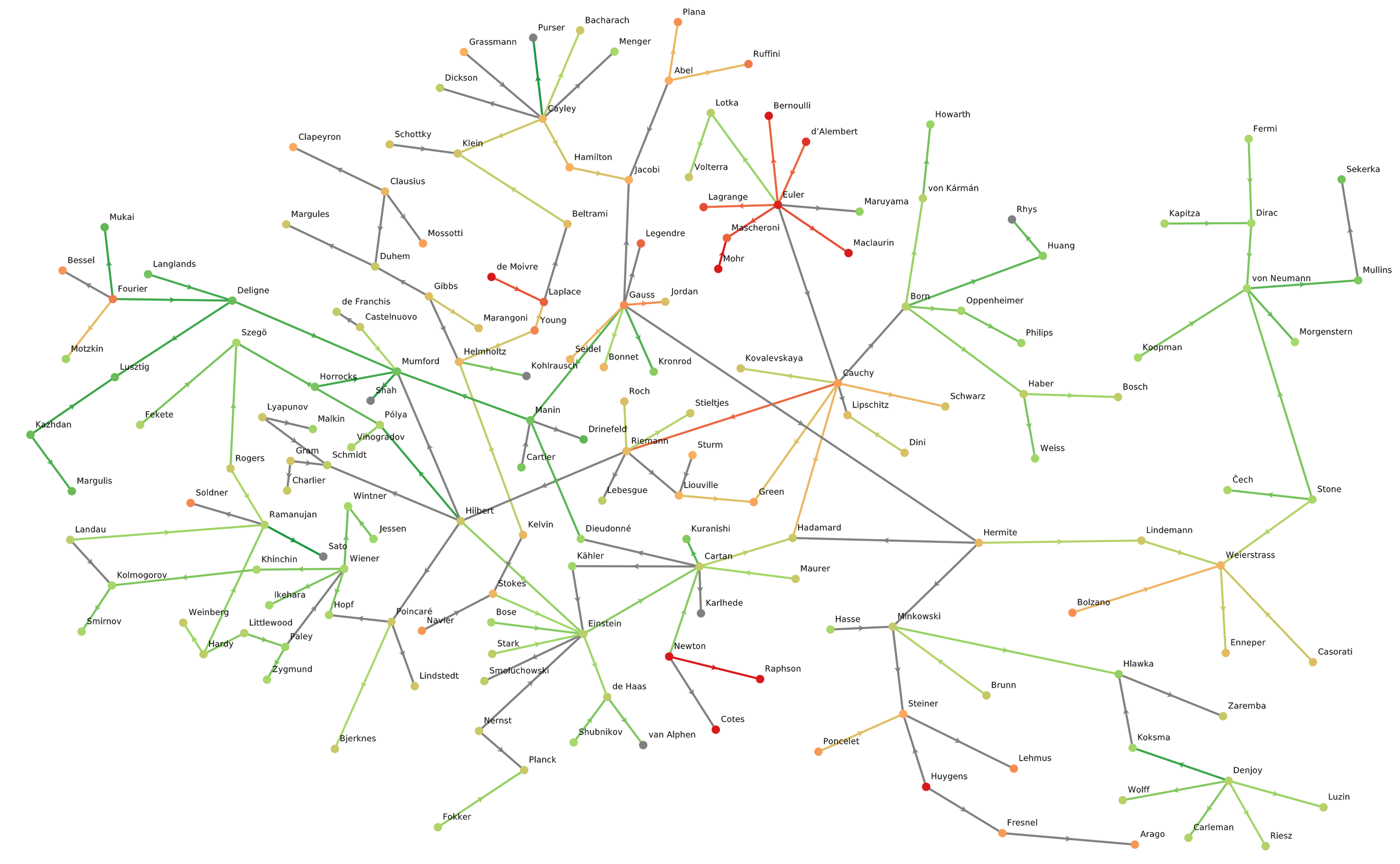
Here’s a first visualization of the graph, resulting from the command plot_graph(node_color_prop="birth_year", edge_color_prop = "year"). It uses one unified color scheme, ranging from red to green, to indicate the birth years of people at the nodes, and the year of reference for the theories on the edges:

There are a lot of isolated clusters here, which make things hard to reason about. Let’s get just the largest connected cluster…

julia> cs = get_clusters() # get all connected clusters
 [1, 4, 6, 12, 15, 18, 21, 26, 27, 28  …  419, 427, 428, 430, 435, 437, 441, 443, 444, 446]
 [13, 57, 80, 106, 113, 121, 124, 165, 200, 239  …  298, 314, 315, 325, 333, 340, 350, 359, 381, 403]
 [2, 19, 55, 101, 125, 140, 146, 190, 201, 203, 205, 218, 276, 305, 351, 358, 374, 423]
 [8, 9, 16, 88, 149, 170, 254, 287, 328, 352, 367, 383, 398, 399, 402]
 [32, 51, 151, 171, 187, 221, 230, 275, 310, 311, 343, 408, 413]
 [63, 112, 152, 216, 225, 229, 265, 332, 382, 396, 442, 445]
 [5, 127, 175, 179, 181, 346, 363, 373]
 [10, 47, 83, 184, 263, 300, 324, 356]
 [195, 227, 271, 274, 301, 318, 376, 406]
 ⋮
 [294, 429]
 [307, 432]
 [308, 394]
 [322, 345]
 [327, 371]
 [349, 405]
 [375, 440]
 [393, 438]
 [395, 424]

julia> sg = hg[cs[1]] # could also do trim_graph(threshold=100)
HyphenGraph with 248 people, 251 hyphens

julia> julia> plot_graph(sg, node_color_prop="birth_year", edge_color_prop="year")

The GLMakie visualization is interactive, so I did some manual rearranging of the node positions to make this more visually parse-able…see “how you can help” below).

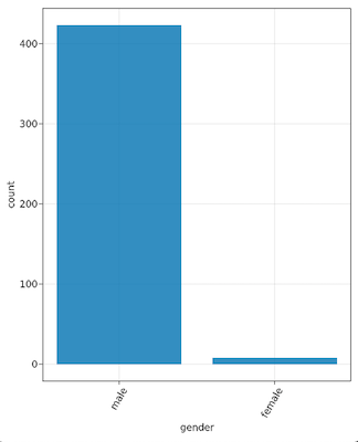
We could also color nodes by other properties such as various demographic properties, but some of those are a bit easier to parse if we just look at some histograms. For that, there’s a node_histogram function. For example, node_histogram(“gender”) yields:

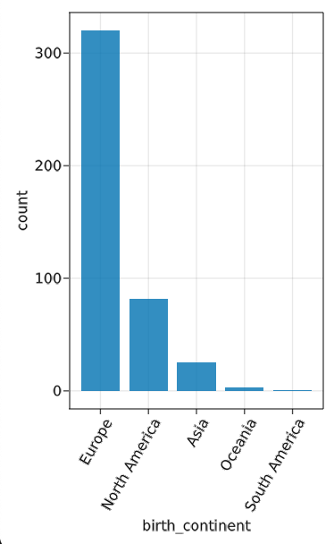
Pretty depressing. Even more so if you then try node_histogram(“given_name”), at which point you can find which three male names have more instances than the total number of women. Similar results from node_histogram("birth_continent")…

Obviously, a lot of this reflects historical norms and precedents, but it’s a pretty dramatic representation of how we can and need to do better going forward as a community. (It also, perhaps, suggests opportunities for targeted Wikipedia content-creation campaigns!)

But let’s try something else fun! Because HyphenGraph<:AbstractGraph, lots of LightGraphs functionality “just works” here (in fact we’ve already used it to find clusters above), so we can do neat stuff like probe centrality measures. I’ve included some functions for this:

julia> most_central(betweenness_centrality) # get details for one measure
Dict{Symbol, Any} with 9 entries:
  :birth_year      => 1879
  :given_name      => "Albert"
  :death_year      => 1955
  :birth_country   => "Germany"
  :race            => "white"
  :reference       => "https://en.wikipedia.org/wiki/Albert_Einstein"
  :birth_continent => "Europe"
  :family_name     => "Einstein"
  :gender          => "male"

julia> all_centrals() # or just do a bunch of them!
betweenness_centrality: Albert Einstein
closeness_centrality: Leonhard Euler
degree_centrality: Albert Einstein
eigenvector_centrality: Satyendra Bose
katz_centrality: David Mumford
pagerank: Albert Einstein
stress_centrality: Albert Einstein
radiality_centrality: Niels Abel

Or, we can answer the question that started it all…

julia> paths = longest_path() # get indices of paths
2-element Vector{Vector{Int64}}:
 [183, 391, 82, 40, 75, 248, 282, 368]
 [285, 391, 82, 40, 75, 248, 282, 368]

julia> hg[paths[1]].node_info.family_name
8-element Vector{String}:
 "Kelvin"
 "Stokes"
 "Einstein"
 "Cartan"
 "Dieudonné"
 "Manin"
 "Mumford"
 "Shah"

julia> hg[paths[2]].node_info.family_name
8-element Vector{String}:
 "Navier"
 "Stokes"
 "Einstein"
 "Cartan"
 "Dieudonné"
 "Manin"
 "Mumford"
 "Shah"

How can you help?

In plenty of ways! Some ideas to start with:

1. Add more data! The best way to do this is by GitHub pull request. While it’s not absolutely required, I would strongly request that if you do this, you follow these guidelines:
   1. Chase tails thoroughly. e.g. if you want to add the A-B theorem, but A is also part of the A-C conjecture, the D-A algorithm, etc., make sure to add those (and so on down the branches).
   2. Add as much data as you can find (leave minimal missing entries in the CSV files); try to at least exhaust Wikipedia’s resources.
   3. Please include open-access references in those fields.
2. Help with graph layout! You may notice that there are lots of edge crossings in the plots above. I’ve played around with a variety of layout algorithms from the NetworkLayout.jl package, but none of them are quite satisfactory. If you’re handy with that sort of thing, feel free to help!
3. Other visualization help! I have an alternative approach to graph visualization that you can see at Nodariety (GitHub repo here) that has some nice things about it; in particular the little popups with other information. Would be cool to figure out a non-laggy way to do that within GraphMakie…
4. Try out other fun ideas for graph analysis and make PR’s with those functions!

I very much hope people might find this as rewarding of a hobby pursuit as I’ve found it to be, and would very much welcome any and all contributions! Please check out the issues on the repository for some more specific suggestions, as well!